23 Probability with tables
Coming soon!
23.1 Defining probability
A random process is one in which the outcome is unpredictable. We encounter random processes every day: will it rain today? how many minutes will pass until receiving your next text message? will the Seahawks win the Super Bowl? Though the outcome of one particular random process is unpredictable, if we observe the process many many times, the pattern of outcomes, or its probability distribution, can often be modeled mathematically. Though there are several philosophical definitions of probability, we will use the “frequentist” definition of probability—a long-run relative frequency.
Probability.
The probability of an event is the long-run proportion of times the event would occur if the random process were repeated indefinitely (under identical conditions).
Consider the simple example of flipping a fair coin once. What is the probability the coin lands on heads. From its physical properties, we assume the probability of heads is 0.5, but let’s use simulation to examine the probability. Figure 23.1 shows the long-run proportion of times a simulated coin flip lands on heads on the y-axis, and the number of tosses on the x-axis. Notice how the long-run proportion starts converging to 0.5 as the number of tosses increases.
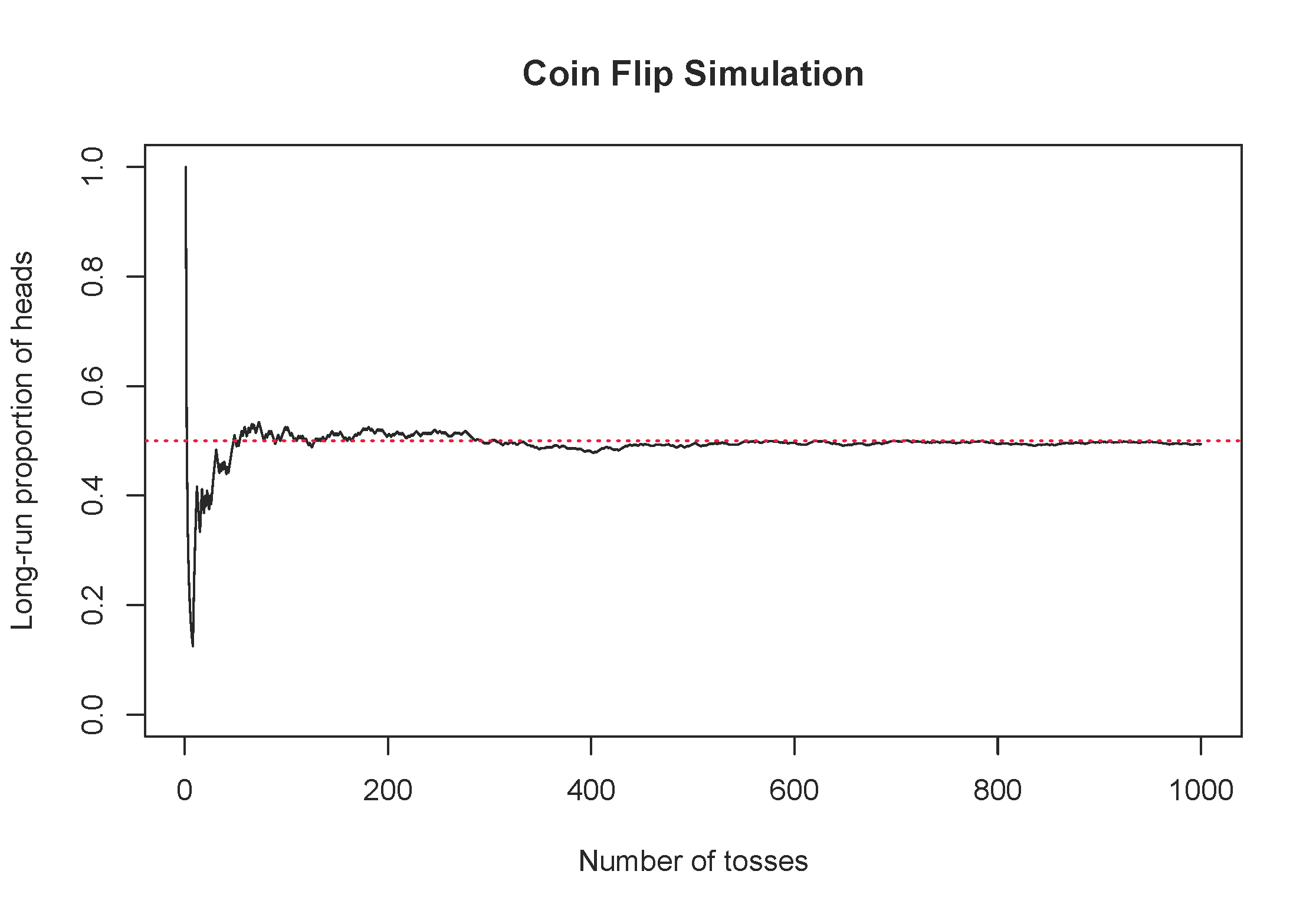
Figure 23.1: One simulation of flipping a fair coin, tracking the long-run proportion of times the coin lands on heads.
23.2 Finding probabilities with tables
We can solve many real-life probability problems without using any equations by creating a hypothetical two-way table of the scenario. This tool is best demonstrated by an example.
As a student at Montana State University, suppose your first class on Mondays is in Wilson Hall at 8:00am and you commute to school. You have a Bobcat parking permit. From past experience, you know that there is a 20% chance of finding an open parking spot in Lot 6 by Animal Bioscience. Otherwise, you have to park in Lot 18 by graduate housing. If you find a spot in Lot 6, you only have a 5% chance of being late to class. However, if you have to park in Lot 18, you have a 15% chance of being late to class. What is the probability that you will be late to class this Monday?
There are two random variables in this scenario: whether you park in Lot 6 or Lot 18, and whether or not you are late to class. Since we know probability is a long-run relative frequency, let’s imagine 1000 hypothetical Mondays, and fill in a contingency table with the frequencies we’d expect in each cell.
| Late to class | Not late to class | Total | |
|---|---|---|---|
| Lot 6 | 10 | 190 | 200 |
| Lot 18 | 120 | 680 | 800 |
| Total | 130 | 870 | 1000 |
Now we can find the probability of being late to class by reading it off the table: 130/1000 = 0.13.
How did we create the table in the last Example? Let’s work through it step-by-step.
- Identify the unconditional probabilities given in the problem: 20% chance of parking in Lot 6, which means an 80% chance of parking in Lot 18. Take 20% and 80% of 1000 to fill in the row totals:
| Late to class | Not late to class | Total | |
|---|---|---|---|
| Lot 6 | 1000 \(\times\) 0.20 = 200 | ||
| Lot 18 | 1000 \(\times\) 0.80 = 800 | ||
| Total | 1000 |
- Identify the conditional probabilities given in the problem: if you park in Lot 6, the probability of being late to class is 5%; if you park in Log 18, the probability of being late to class is 15%. Fill in the corresponding cells in the table by taking 5% of the times you parked in Lot 6, and 15% of the times you parked in Lot 18:
| Late to class | Not late to class | Total | |
|---|---|---|---|
| Lot 6 | 200 \(\times\) 0.05 = 10 | 200 | |
| Lot 18 | 800 \(\times\) 0.15 = 120 | 800 | |
| Total | 1000 |
- Use subtraction to fill in the remaining cells for the column “Not late to class.” Use addition to find the column totals.
Using the hypothetical two-way table given in the last Example, find the following probabilities:
- What is the probability you are not late to class?
- What is the probability that you park in Lot 6 and you are not late to class?
- Given that you were late to class, what is the probability you parked in Lot 18?166
Carefully read how each of the probabilities is described in the Guided Practice—note the subtle difference between “the probability of being late to class, given that you parked in Lot 18” (\(120/800 = 0.15\)) and “the probability of parking in Lot 18, given that you were late to class” (\(120/130 = 0.923\)). When we are given extra information, this is called a conditional probability, and the denominator in the probability calculation is a row total (e.g., 800) or column total (e.g., 130) rather than the overall total in the hypothetical two-way table.
In the previous Guided Practice, which of the probabilities are conditional probabilities? which are unconditional?167
23.3 Probability notation
For ease of translating probability problems into calculations, let’s define some notation. We will denote “events” (e.g., being late to class) by upper case letters near the beginning of the alphabet, e.g., \(A\), \(B\), \(C\). The probability of an event \(A\) will be denoted by \(P(A)\), so \(P(A)\) is a number between 0 and 1. The event that \(A\) does not happen is called the complement of \(A\) and is denoted by \(P(A^C)\). Sometimes we have additional information that we would like to condition on, and we denote the conditional probability of \(A\) given \(B\) by \(P(A | B)\)—the probability that \(A\) happens given that \(B\) has already happened.
In our coin flip example, we could let \(A\) be the event that the coin lands on heads. Then we can denote the probability that the coin lands on heads by \(P(A) = 0.5\). We could flip the coin twice and let \(H_1\) be the event that the first flip lands on heads, and \(H_2\) be the event that the second flip lands on heads. Since the coin does not remember its last flip, if the first flip lands on heads, the second flip still has a 50% chance of landing on heads. That is, \(P(H_2 | H_1) = 0.5\).
23.4 Diagnostic testing
Medical diagnostic tests for diseases spend years in development. Through clinical trials, developers of the diagnostic test are able to determine two important properties of the test:
- The sensitivity of a diagnostic test is the probability the test yields a positive result, given the individual has the disease. In other words, what proportion of the diseased population would test positive?
- The specificity of the diagnostic test is the probability the test yields a negative result, given the individual does not have the disease. That is, what proportion of the non-diseased population would test negative?
A good diagnostic test has very high (near 100%) sensitivity and specificity. However, even for a near-perfect test, the probability that you have the disease given you test positive could still be quite low. To investigate this counter-intuitive result, we need another definition:
- We will call the proportion of the population that has the disease—the probability of contracting the disease—the prevalence (incidence) of a disease.
Let \(D\) be the event that an individual has the disease and \(T\) be the event that an individual tests positive. How would you express each of the following quantities using probability notation?
- sensitivity
- specificity
- prevalence168
Note that sensitivity and specificity are conditional probabilities, while prevalence is an unconditional probability. While the above probabilities are useful information, if you test positive on a diagnostic test, none of these quantities is the probability you really want to know: the conditional probability of having the disease, given you tested positive, \(P(D | T)\).
23.4.1 The case of Baby Jeff
The following case study was presented by Slawson and Shaughnessy (2002). A poster in a hospital’s newborn nursery announced that all male newborns would be screened for muscular dystrophy using a heel stick blood test for creatinine phosphokinase (CPK). The test characteristics of the screening tests were nearly perfect: a sensitivity of 100% and a specificity of 99.98%. The prevalence of muscular dystrophy in male newborns ranges from 1 in 3,500 to 1 in 15,000. Baby Jeff had an abnormal CPK test. The parents of the baby wanted to know, “What is the chance that our son has muscular dystrophy?” Doctors informed the parents that though not 100% likely, it was highly probable. First, take a minute and predict this probability – what do you think? 80% chance? 99% chance? Let’s investigate using a two-way table of a hypothetical population of 100,000 male newborns.
For our calculations, let’s use a prevalence of 1 in 10,000. Then out of 100,000 hypothetical male newborns, we would expect 1 in 10,000 to have muscular dystrophy, or 10: \((1/10000)\times 100000 = 10\). The sensitivity of the test is perfect, so all 10 of the male newborns with muscular dystrophy will test positive. Of the \(100000-10 = 99,990\) male newborns that do not have muscular dystrophy, 99.98% will test negative: \((0.9998)\times 99990 = 99,970\) infants. That leaves \(99990 - 99970 = 20\) male newborns that test positive even though they do not have muscular dystrophy. This allows us to fill in the counts in our hypothetical two-way table:
| Tests positive | Tests negative | Total | |
|---|---|---|---|
| Has muscular dystrophy | 10 | 0 | 10 |
| Does not have muscular dystrophy | 20 | 99,970 | 99,990 |
| Total | 30 | 99,970 | 100,000 |
Now we can read off the desired probability from the table: of the 30 male newborns we’d expect to test positive, only 10 of them actually have muscular dystrophy. This means the chance Baby Jeff has muscular dystrophy is only about 33%!
How would this probability change if the prevalence were 1/3500? 1/15000? Try it.169
Why did this counter-intuitive result occur? With such high sensitivity and specificity, why does this test perform so poorly? The answer has to do with the prevalence of the disease. For a rare disease, the very small proportion that test positive out of the very large group of people without the disease will overwhelm the very large proportion that test positive out of the very small group of people with the disease. The number of false positives can be much higher than the number of true positives.
23.5 Chapter review
Terms
We introduced the following terms in the chapter. If you’re not sure what some of these terms mean, we recommend you go back in the text and review their definitions. We are purposefully presenting them in alphabetical order, instead of in order of appearance, so they will be a little more challenging to locate. However you should be able to easily spot them as bolded text.
| probability | random process |
Key ideas
Probabilities can be either unconditional or conditional. An unconditional probability or proportion is a proportion measured on the entire population; whereas a conditional probability or proportion is a proportion measured on a subgroup of the population. When computing probabilities using a contingency table, unconditional probabilities are computed by dividing a cell total by the overall total; conditional probabilities are computed by dividing a cell total by a row or column total.
Recall from Chapter 4 that two variables are associated when the behavior of one variable depends on the value of the other variable. For two categorical variables, this occurs when some or all of the conditional probabilities in each category of one variable change across probabilities of the other variable.